
Continuous Delivery for Machine Learning
Automating the end-to-end lifecycle of Machine Learning applications
Machine Learning applications are becoming popular in our industry, however the process for developing, deploying, and continuously improving them is more complex compared to more traditional software, such as a web service or a mobile application. They are subject to change in three axis: the code itself, the model, and the data. Their behaviour is often complex and hard to predict, and they are harder to test, harder to explain, and harder to improve. Continuous Delivery for Machine Learning (CD4ML) is the discipline of bringing Continuous Delivery principles and practices to Machine Learning applications.
19 September 2019

bio
I am a principal consultant at Thoughtworks with experience in many areas of architecture and engineering: software, data, infrastructure, and machine learning. I am the author of DevOps in Practice: Reliable and Automated Software Delivery, a member of Thoughtworks Technology Advisory Board, and Thoughtworks Office of the CTO.

bio
I am a consultant at Thoughtworks Germany, where I am leading our data and machine learning activities. I enjoy building scalable software that makes an impact — and building teams that create such software. I am particularly fascinated about how effectively building ML applications requires data scientists and developers (like myself) to work closely together.

bio
I am a principal consultant at Thoughtworks and the global lead for Intelligent Empowerment. I am helping our clients and Thoughtworks to create value with the latest technologies in AI and machine learning. After finishing my Ph.D. in Neural Networks I spend 20+ years in the IT industry. I am a member of the Thoughtworks Office of the CTO.
Introduction and Definition
In the famous Google paper published by Sculley et al. in 2015 “Hidden Technical Debt in Machine Learning Systems”, they highlight that in real-world Machine Learning (ML) systems, only a small fraction is comprised of actual ML code. There is a vast array of surrounding infrastructure and processes to support their evolution. They also discuss the many sources of technical debt that can accumulate in such systems, some of which are related to data dependencies, model complexity, reproducibility, testing, monitoring, and dealing with changes in the external world.
Many of the same concerns are also present in traditional software systems, and Continuous Delivery has been the approach to bring automation, quality, and discipline to create a reliable and repeatable process to release software into production.
In their seminal book “Continuous Delivery”, Jez Humble and David Farley state that:
“Continuous Delivery is the ability to get changes of all types — including new features, configuration changes, bug fixes, and experiments — into production, or into the hands of users, safely and quickly in a sustainable way”.
Besides the code, changes to ML models and the data used to train them are another type of change that needs to be managed and baked into the software delivery process (Figure 1).
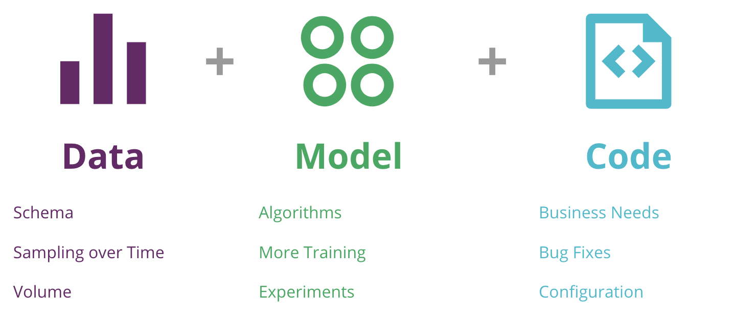
Figure 1: the 3 axis of change in a Machine Learning application — data, model, and code — and a few reasons for them to change
With that in mind, we can extend the Continuous Delivery definition to incorporate the new elements and challenges that exist in real-world Machine Learning systems, an approach we are calling “Continuous Delivery for Machine Learning (CD4ML)”.
Continuous Delivery for Machine Learning (CD4ML) is a software engineering approach in which a cross-functional team produces machine learning applications based on code, data, and models in small and safe increments that can be reproduced and reliably released at any time, in short adaptation cycles.
This definition contains all the basic principles:
Software engineering approach: It enables teams to efficiently produce high quality software.
Cross-functional team: Experts with different skill sets and workflows across data engineering, data science, machine learning engineering, development, operations, and other knowledge areas are working together in a collaborative way emphasizing the skills and strengths of each team member.
Producing software based on code, data, and machine learning models: All artifacts of the ML software production process require different tools and workflows that must be versioned and managed accordingly.
Small and safe increments: The release of the software artifacts is divided into small increments, which allows visibility and control around the levels of variance of its outcomes, adding safety into the process.
Reproducible and reliable software release: While the model ouputs can be non-deterministic and hard to reproduce, the process of releasing ML software into production is reliable and reproducible, leveraging automation as much as possible.
Software release at any time: It is important that the ML software could be delivered into production at any time. Even if organizations do not want to deliver software all the time, it should always be in a releasable state. This makes the decision about when to release it a business decision rather than a technical one.
Short adaptation cycles: Short cycles means development cycles are in the order of days or even hours, not weeks, months or even years. Automation of the process with quality built in is key to achieve this. This creates a feedback loop that allows you to adapt your models by learning from its behavior in production.
In this article, we will describe the technical components we found important when implementing CD4ML, using a sample ML application to explain the concepts and demonstrate how different tools can be used together to implement the full end-to-end process. Where appropriate, we will highlight alternative tool choices to the ones we selected. We will also discuss further areas of development and research, as the practice matures across our industry.
A Machine Learning Application for Sales Forecasting
We have started thinking about how to apply Continuous Delivery to Machine Learning systems since 2016, and we published and presented a case study from a client project we built with AutoScout to predict the pricing for cars that were published in their platform.
However, we have decided to build a sample ML application based on a public problem and dataset to illustrate a CD4ML implementation, as we are not allowed to use examples from real client code. This application solves a common forecasting problem faced by many retailers: trying to predict how much of a given product will sell in the future, based on historical data. We built a simplified solution to a Kaggle problem posted by Corporación Favorita, a large Ecuadorian-based grocery retailer. For our purposes, we have combined and simplified their data sets, as our goal is not to find the best predictions — a job better handled by your Data Scientists — but to demonstrate how to implement CD4ML.
Using a supervised learning algorithm and the popular scikit-learn Python library, we train a prediction model using the labeled input data, integrate that model into a simple web application, which are then deployed to a production environment in the cloud. Figure 2 shows the high-level process.
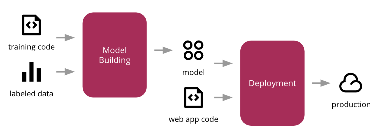
Figure 2: initial process to train our ML model, integrate it with a web application, and deploy into production
Once deployed, our web application (Figure 3) allows users to select a product and a date in the future, and the model will output its prediction of how many units of that product will be sold on that day.
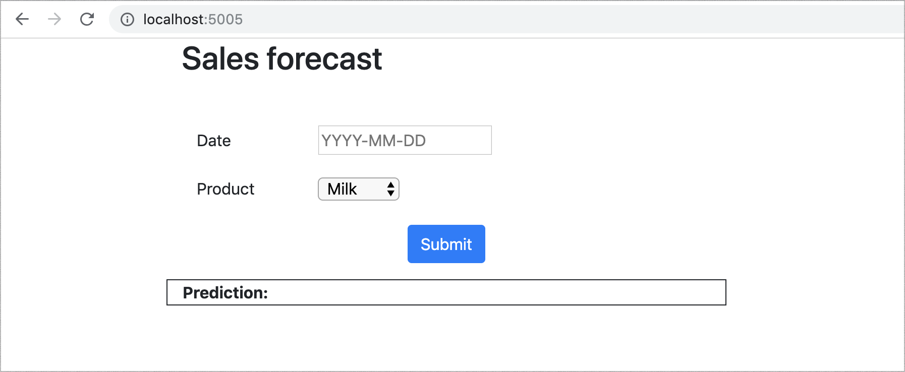
Figure 3: the web UI to demonstrate our model in action
Common challenges
While this is a good starting point for our discussion, implementing this process end-to-end can already present two challenges. The first challenge is the organizational structure: different teams might own different parts of the process, and there is a hand over — or usually, “throw over the wall” — without clear expectations of how to cross these boundaries (Figure 4). Data Engineers might be building pipelines to make data accessible, while Data Scientists are worried about building and improving the ML model. Then Machine Learning Engineers or developers will have to worry about how to integrate that model and release it to production.
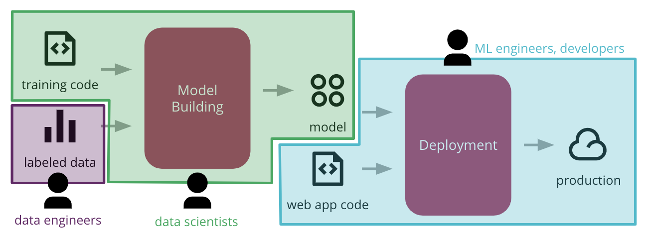
Figure 4: common functional silos in large organizations can create barriers, stifling the ability to automate the end-to-end process of deploying ML applications to production
This leads to delays and friction. A common symptom is having models that only work in a lab environment and never leave the proof-of-concept phase. Or if they make it to production, in a manual ad-hoc way, they become stale and hard to update.
The second challenge is technical: how to make the process reproducible and auditable. Because these teams use different tools and follow different workflows, it becomes hard to automate it end-to-end. There are more artifacts to be managed beyond the code, and versioning them is not straightforward. Some of them can be really large, requiring more sophisticated tools to store and retrieve them efficiently.
Solving the organizational challenge is outside the scope of this article, but we can bring our learnings from Agile and DevOps and build cross-functional and Outcome Oriented teams that include specialists from different disciplines to deliver an end-to-end ML system. If that is not possible in your organization, at least encourage breaking down those barriers and have them collaborate early and often throughout the process.
The remainder of this article will explore solutions we found for the technical challenges. We will deep dive into each technical component, as well as slowly improve and extend the end-to-end process to make it more robust.
Technical Components of CD4ML
As we considered how to solve the forecasting problem using Machine Learning, the first step was to understand the data set. In this case, it was a collection of CSV files, containing information about:
- the products, like their categorization and whether they are perishable or not
- the stores, like their location and how they are clustered together
- special events, like public holidays, seasonal events, or a 7.8 magnitude earthquake that struck Ecuador in 2016
- the sales transactions, including the number of units sold for a given product, date, and location
At this stage, Data Analysts and Data Scientists will usually perform some sort of Exploratory Data Analysis (EDA) to understand the shape of the data, and identify broad patterns and outliers. As an example, we found products with a negative number of units sold, which we interpreted as returns. As we only intended to explore sales, and not returns, we removed them from our training dataset.
In many organizations, the data required to train useful ML models, will likely not be structured exactly the way a Data Scientist might need, therefore it highlights the first technical component: discoverable and accessible data.
Discoverable and Accessible Data
The most common source of data will be your core transactional systems. However, there is also value in bringing other data sources from outside your organization. We have found a few common patterns for collecting and making data available, like using a Data Lake architecture, a more traditional data warehouse, a collection of real-time data streams, or more recently, we are experimenting with a decentralized Data Mesh architecture.
Regardless of which flavour of architecture you have, it is important that the data is easily discoverable and accessible. The harder it is for Data Scientists to find the data they need, the longer it will take for them to build useful models. We should also consider they will want to engineer new features on top of the input data, that might help improve their model's performance.
In our example, after doing the initial Exploratory Data Analysis, we decided to de-normalize multiple files into a single CSV file, and cleanup the data points that were not relevant or that could introduce unwanted noise into the model (like the negative sales). We then stored the output in a cloud storage system like Amazon S3, Google Cloud Storage, or Azure Storage Account.
Using this file to represent a snapshot of the input training data, we are able to devise a simple approach to version our dataset based on the folder structure and file naming conventions. Data versioning is an extensive topic, as it can change in two different axis: structural changes to its schema, and the actual sampling of data over time. Our Data Scientist, Emily Gorcenski, covers this topic in more detail on this blog post, but later in the article we will discuss other ways to version datasets over time.
It is worth noting that, in the real world, you will likely have more complex data pipelines to move data from multiple sources into a place where it can be accessed and used by Data Scientists.
Reproducible Model Training
Once the data is available, we move into the iterative Data Science workflow of model building. This usually involves splitting the data into a training set and a validation set, trying different combinations of algorithms, and tuning their parameters and hyper-parameters. That produces a model that can be evaluated against the validation set, to assess the quality of its predictions. The step-by-step of this model training process becomes the machine learning pipeline.
In Figure 5 we show how we structured the ML pipeline for our sales forecasting problem, highlighting the different source code, data, and model components. The input data, the intermediate training and validation data sets, and the output model can potentially be large files, which we don't want to store in the source control repository. Also, the stages of the pipeline are usually in constant change, which makes it hard to reproduce them outside of the Data Scientist's local environment.
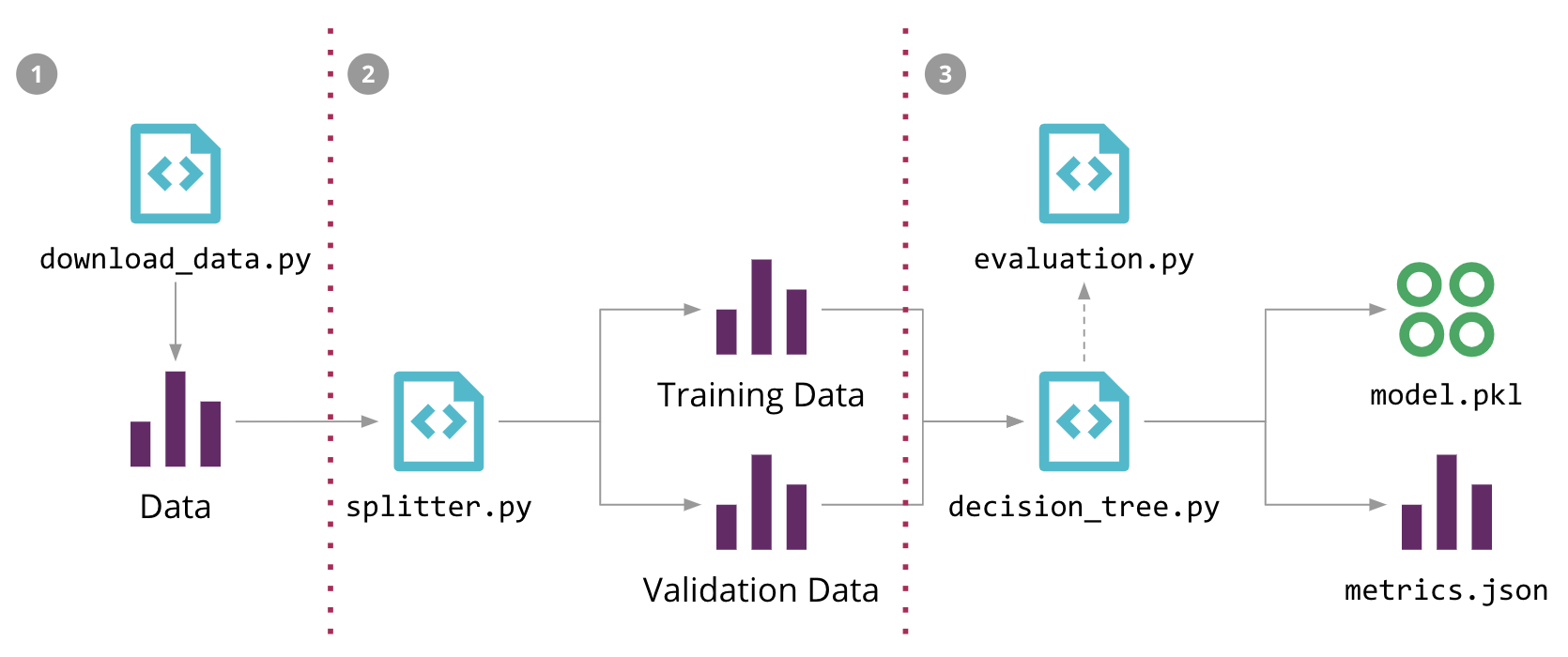
Figure 5: Machine Learning pipeline for our Sales Forecasting problem, and the 3 steps to automate it with DVC
In order to formalise the model training process in code, we used an open source tool called DVC (Data Science Version Control). It provides similar semantics to Git, but also solves a few ML-specific problems:
- it has multiple backend plugins to fetch and store large files on an external storage outside of the source control repository;
- it can keep track of those files' versions, allowing us to retrain our models when the data changes;
- it keeps track of the dependency graph and commands used to execute the ML pipeline, allowing the process to be reproduced in other environments;
- it can integrate with Git branches to allow multiple experiments to co-exist;
For example, we can configure our initial ML pipeline in Figure 5 with three dvc run commands
(-d specify dependencies, -o specify outputs,
-f is the filename to record that step, and -M
is the resulting metrics):
dvc run -f input.dvc \ ➊
  -d src/download_data.py -o data/raw/store47-2016.csv python src/download_data.py
dvc run -f split.dvc \ ➋
  -d data/raw/store47-2016.csv -d src/splitter.py \
  -o data/splitter/train.csv -o data/splitter/validation.csv python src/splitter.py
dvc run ➌
  -d data/splitter/train.csv -d data/splitter/validation.csv -d src/decision_tree.py \
  -o data/decision_tree/model.pkl -M results/metrics.json python src/decision_tree.py
Each run will create a corresponding file, that can be committed to
version control, and that allows other people to reproduce the entire ML
pipeline, by executing the dvc repro command.
Once we find a suitable model, we will treat it as an artifact that
needs to be versioned and deployed to production. With DVC, we can use
the dvc push and dvc pull commands to publish
and fetch it from external storage.
There are other open source tools that you can use to solve these problems: Pachyderm uses containers to execute the different steps of the pipeline and also solves the data versioning and data provenance issues by tracking data commits and optimizing the pipeline execution based on that. MLflow Projects defines a file format to specify the environment and the steps of the pipeline, and provides both an API and a CLI tool to run the project locally or remotely. We chose DVC because it is a simple CLI tool that solves this part of the problem very well.
Model Serving
Once a suitable model is found, we need to decide how it will be served and used in production. We have seen a few patterns to achieve that:
- Embedded model: this is the simpler approach, where you treat the model artifact as a dependency that is built and packaged within the consuming application. From this point forward, you can treat the application artifact and version as being a combination of the application code and the chosen model.
- Model deployed as a separate service: in this approach, the model is wrapped in a service that can be deployed independently of the consuming applications. This allows updates to the model to be released independently, but it can also introduce latency at inference time, as there will be some sort of remote invocation required for each prediction.
- Model published as data: in this approach, the model is also treated and published independently, but the consuming application will ingest it as data at runtime. We have seen this used in streaming/real-time scenarios where the application can subscribe to events that are published whenever a new model version is released, and ingest them into memory while continuing to predict using the previous version. Software release patterns such as Blue Green Deployment or Canary Releases can also be applied in this scenario.
In our example, we have decided to use the simpler approach of embedding the model, given our consuming application is also written in Python. Our model is exported as a serialized object (pickle file) and pushed to storage by DVC. When building our application, we pull it and embed it inside the same Docker container. From that point onwards, the Docker image becomes our application+model artifact that gets versioned and deployed to production.
There are other tool options to implement the embedded model pattern, besides serializing the model object with pickle. MLeap provides a common serialization format for exporting/importing Spark, scikit-learn, and Tensorflow models. There are also language-agnostic exchange formats to share models, such as PMML, PFA, and ONNX. Some of these serialization options are also applicable for implementing the “model as data” pattern.
Another approach is to use a tool like H2O to export the model as a POJO in a JAR Java library, which you can then add as a dependency in your application. The benefit of this approach is that you can train the models in a language familiar to Data Scientists, such as Python or R, and export the model as a compiled binary that runs in a different target environment (JVM), which can be faster at inference time.
To implement the “model as service” pattern, many of the cloud providers have tools and SDKs to wrap your model for deployment into their MLaaS (Machine Learning as a Service) platforms, such as Azure Machine Learning, AWS Sagemaker, or Google AI Platform. Another option is to use a tool like Kubeflow, which is a project designed to deploy ML workflows on Kubernetes, although it tries to solve more than just the model serving part of the problem.
MLflow Models is trying to provide a standard way to package models in different flavours, to be used by different downstream tools, some in the “model as a service”, some in the “embedded model” pattern. Suffice to say, this is a current area of development and various tools and vendors are working to simplify this task. But it means there is no clear standard (open or proprietary) that can be considered a clear winner yet, and therefore you will need to evaluate the right option for your needs.
It is worth noting that, regardless of which pattern you decide to use, there is always an implicit contract between the model and its consumers. The model will usually expect input data in a certain shape, and if Data Scientists change that contract to require new input or add new features, you can cause integration issues and break the applications using it. Which leads us to the topic of testing.
Testing and Quality in Machine Learning
There are different types of testing that can be introduced in the ML workflow. While some aspects are inherently non-deterministic and hard to automate, there are many types of automated tests that can add value and improve the overall quality of your ML system:
- Validating data: we can add tests to validate input data against the expected schema, or to validate our assumptions about its valid values — e.g. they fall within expected ranges, or are not null. For engineered features, we can write unit tests to check they are calculated correctly — e.g. numeric features are scaled or normalized, one-hot encoded vectors contain all zeroes and a single 1, or missing values are replaced appropriately.
- Validating component integration: we can use a similar approach to testing the integration between different services, using Contract Tests to validate that the expected model interface is compatible with the consuming application. Another type of testing that is relevant when your model is productionized in a different format, is to make sure that the exported model still produces the same results. This can be achieved by running the original and the productionized models against the same validation dataset, and comparing the results are the same.
- Validating the model quality: While ML model performance is non-deterministic, Data Scientists usually collect and monitor a number of metrics to evaluate a model's performance, such as error rates, accuracy, AUC, ROC, confusion matrix, precision, recall, etc. They are also useful during parameter and hyper-parameter optimization. As a simple quality gate, we can use these metrics to introduce Threshold Tests or ratcheting in our pipeline, to ensure that new models don't degrade against a known performance baseline.
- Validating model bias and fairness: while we might get good performance on the overall test and validation datasets, it is also important to check how the model performs against baselines for specific data slices. For instance, you might have inherent bias in the training data where there are many more data points for a given value of a feature (e.g. race, gender, or region) compared to the actual distribution in the real world, so it's important to check performance across different slices of the data. A tool like Facets can help you visualize those slices and the distribution of values across the features in your datasets.
In our example application, the evaluation metric defined by Favorita is a normalized error rate. We wrote a simple PyUnit threshold test that breaks if the error rate goes above 80%, and this test can be executed prior to publishing a new model version, to demonstrate how we can prevent a bad model from getting promoted.
While these are examples of tests that are easier to automate, assessing a model's quality more holisticaly is harder. Over time, if we always compute metrics against the same dataset, we can start overfitting. And when you have other models already live, you need to ensure that the new model version will not degrade against unseen data. Therefore, managing and curating test data becomes more important 2.
2: There is active research on tools and systems such as ease.ml/ci and ease.ml/meter to help manage and understand when new test data is required, or when models are overfitting.
When models are distributed or exported to be used by a different application, you can also find issues where the engineered features are calculated differently between training and serving time. An approach to help to catch these types of problems is to distribute a holdout dataset along with the model artifact, and allow the consuming application team to reassess the model's performance against the holdout dataset after it is integrated. This would be the equivalent of a broad Integration Test in traditional software development.
Other types of tests can be also considered, but we think it's also important to add some manual stages into the deployment pipeline, to display information about the model and allow humans to decide if they should be promoted or not. This allows you to model a Machine Learning governance process and introduce checks for model bias, model fairness, or gather explainability information for humans to understand how the model is behaving.
With more types of testing, it will make you rethink the shape of your Test Pyramid: you can consider separate pyramids for each type of artifact (code, model, and data), but also how to combine them, as shown in Figure 6. Overall, testing and quality for ML systems is more complex and should be the subject of another in-depth, independent article.
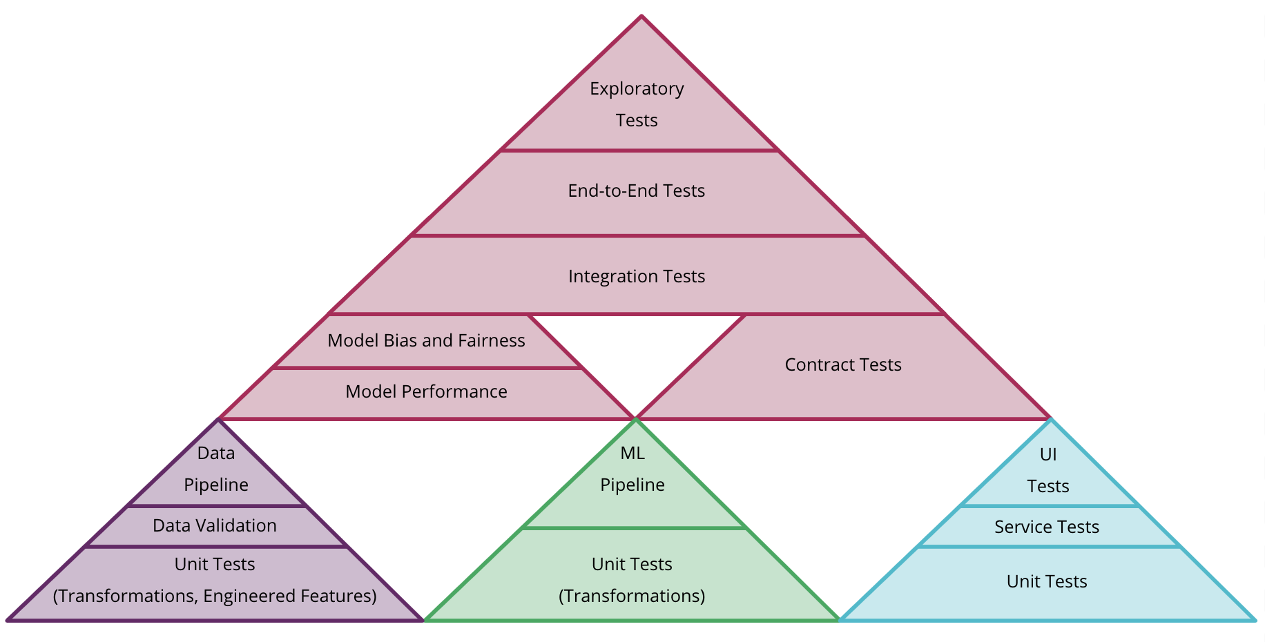
Figure 6: an example of how to combine different test pyramids for data, model, and code in CD4ML
Experiments Tracking
In order to support this governance process, it is important to capture and display information that will allow humans to decide if and which model should be promoted to production. As the Data Science process is very research-centric, it is common that you will have multiple experiments being tried in parallel, and many of them might not ever make it to production.
This experimentation approach during the research phase is different than a more traditional software development process, as we expect that the code for many of these experiments will be thrown away, and only a few of them will be deemed worthy of making it to production. For that reason, we will need to define an approach to track them.
In our case, we decided to follow the approach suggested by DVC, of using different Git branches to track the different experiments in source control. Even though this goes against our preference of practicing Continuous Integration on a single trunk. DVC can fetch and display metrics from experiments running in different branches or tags, making it easy to navigate between them.
Some of the drawbacks of developing in Feature Branches for traditional software development are that it can cause merge pain if the branches are long-lived, it can prevent teams from refactoring more aggressively as the changes can impact broader areas of the codebase, and it hinders the practice of Continuous Integration (CI) as it forces you to setup multiple jobs for each branch and proper integration is delayed until the code is merged back into the mainline.
For ML experimentation, we expect most of the branches to never be integrated, and the variation in the code between experiments is usually not significant. From the CI automation perspective, we actually do want to train multiple models for each experiment, and gather metrics that will inform us which model can move to the next stage of the deployment pipeline.
Besides DVC, another tool we used to help with experiment tracking is MLflow Tracking. It can be deployed as a hosted service, and provides an API and a web interface to visualize the multiple experiment runs, along with their parameters and performance metrics, as shown in Figure 7.
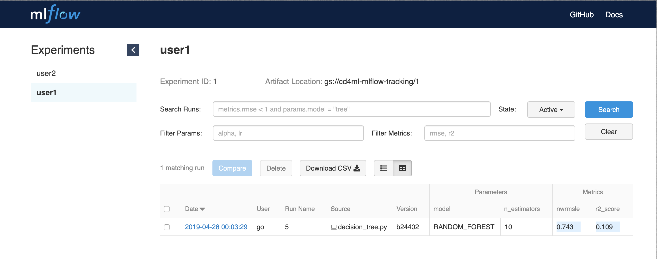
Figure 7: MLflow Tracking web UI to show experiment runs, parameters, and metrics
To support this experimentation process, it is also important to highlight the benefits of having elastic infrastructure, as you might need multiple environments to be available — and sometimes with specialized hardware — for training. Cloud-based infrastructure is a natural fit for this, and many of the public cloud providers are building services and solutions to support various aspects of this process.
Model Deployment
In our simple example, we are only experimenting to build a single model, which gets embedded and deployed with the application. In the real world, deployment might pose more complex scenarios:
- Multiple models: sometimes you might have more than one model performing the same task. For example, we could train a model to predict demand for each product. In that case, deploying the models as a separate service might be better for consuming applications to get predictions with a single API call. And you can later evolve how many models are needed behind that Published Interface.
- Shadow models: this pattern is useful when considering the replacement of a model in production. You can deploy the new model side-by-side with the current one, as a shadow model, and send the same production traffic to gather data on how the shadow model performs before promoting it.
- Competing models: a slightly more complex scenario is when you are trying multiple versions of the model in production — like an A/B test — to find out which one is better. The added complexity here comes from the infrastructure and routing rules required to ensure the traffic is being redirected to the right models, and that you need to gather enough data to make statistically significant decisions, which can take some time. Another popular approach for evaluating multiple competing models is Multi-Armed Bandits, which also requires you to define a way to calculate and monitor the reward associated with using each model. Applying this to ML is an active area of research, and we are starting to see some tools and services appear, such as Seldon core and Azure Personalizer .
- Online learning models: unlike the models we discussed so far, that are trained offline and used online to serve predictions, online learning models use algorithms and techniques that can continuously improve its performance with the arrival of new data. They are constantly learning in production. This poses extra complexities, as versioning the model as a static artifact won't yield the same results if it is not fed the same data. You will need to version not only the training data, but also the production data that will impact the model's performance.
Once again, to support more complex deployment scenarios, you will benefit from using elastic infrastructure. Besides making it possible to run those multiple models in production, it also allows you to improve your system's reliability and scalability by spinning up more infrastructure when needed.
Continuous Delivery Orchestration
With all of the main building blocks in place, there is a need to tie everything together, and this is where our Continuous Delivery orchestration tools come into place. There are many options of tools in this space, with most of them providing means to configure and execute Deployment Pipelines for building and releasing software to production. In CD4ML, we have extra requirements to orchestrate: the provisioning of infrastructure and the execution of the Machine Learning Pipelines to train and capture metrics from multiple model experiments; the build, test, and deployment process for our Data Pipelines; the different types of testing and validation to decide which models to promote; the provisioning of infrastructure and deployment of our models to production.
We chose to use GoCD as our Continuous Delivery tool, as it was built with the concept of pipelines as a first-class concern. Not only that, it also allows us to configure complex workflows and dependencies by combining different pipelines, their triggers, and defining both manual or automated promotion steps between pipeline stages.
In our simplified example, we haven't built any complex Data Pipelines or infrastructure provisioning yet, but we demonstrate how to combine two GoCD pipelines, as shown in Figure 8:
- Machine Learning Pipeline: to perform model training and
evaluation within the GoCD agent, as well as executing the basic
threshold test to decide if the model can be promoted or not. If the
model is good, we perform a
dvc pushcommand to publish it as an artifact. - Application Deployment Pipeline: to build and test the
application code, to fetch the promoted model from the upstream
pipeline using
dvc pull, to package a new combined artifact that contains the model and the application as a Docker image, and to deploy them to a Kubernetes production cluster.
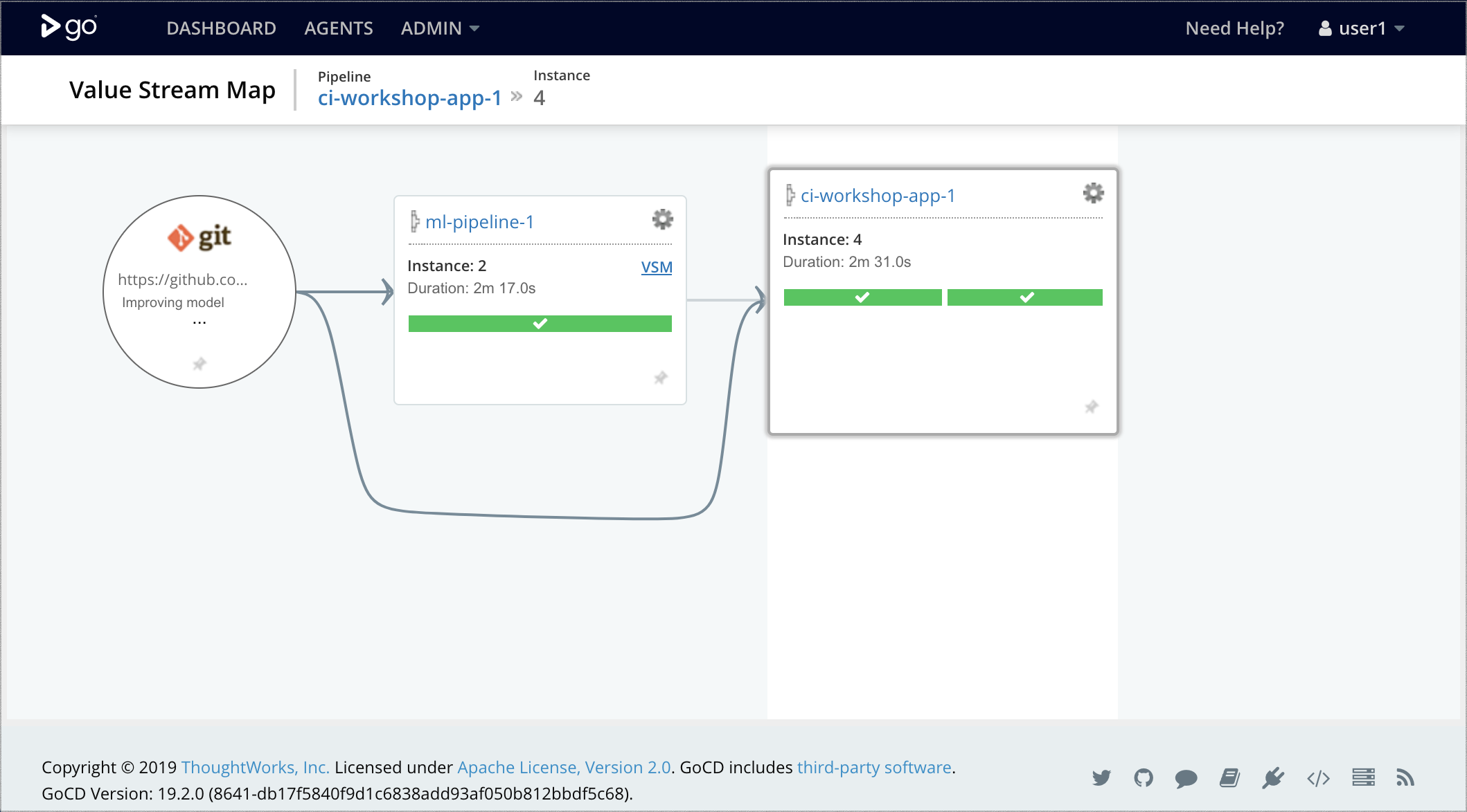
Figure 8: Combining Machine Learning Pipeline and Application Deployment Pipeline in GoCD
Over time, the ML pipeline can be extended to execute multiple experiments in parallel (a feature supported by GoCD's fan-out/fan-in model), and to define your model governance process to check for bias, fairness, correctness, and other types of gates to make informed decisions about which model is promoted and deployed to production.
Finally, another aspect of your Continuous Delivery orchestration is to define a process for rollbacks, in case a deployed model turns out to perform poorly or incorrectly in production. This adds another safety net into the overall process.
Model Monitoring and Observability
Now that the model is live, we need to understand how it performs in production and close the data feedback loop. Here we can reuse all the monitoring and observability infrastructure that might already be in place for your applications and services.
Tools for log aggregation and metrics collection are usually used to capture data from a live system such as business KPIs, software reliability and performance metrics, debugging information for troubleshooting, and other indicators that could trigger alerts when something goes out of the ordinary. We can also leverage these same tools to capture data to understand how our model is behaving such as:
- Model inputs: what data is being fed to the models, giving visibility into any training-serving skew. Model outputs: what predictions and recommendations are the models making from these inputs, to understand how the model is performing with real data.
- Model interpretability outputs: metrics such as model coefficients, ELI5, or LIME outputs that allow further investigation to understand how the models are making predictions to identify potential overfit or bias that was not found during training.
- Model outputs and decisions: what predictions our models are making given the production input data, and also which decisions are being made with those predictions. Sometimes the application might choose to ignore the model and make a decision based on pre-defined rules (or to avoid future bias).
- User action and rewards: based on further user action, we can capture reward metrics to understand if the model is having the desired effect. For example, if we display product recommendations, we can track when the user decides to purchase the recommended product as a reward.
- Model fairness: analysing input data and output predictions against known features that could bias, such as race, gender, age, income groups, etc.
In our example, we are using the EFK stack for monitoring and observability, composed of three main tools:
- Elasticsearch: an open source search engine.
- FluentD: an open source data collector for unified logging layer.
- Kibana: an open source web UI that makes it easy to explore and visualize the data indexed by Elasticsearch.
We can instrument our application code to log the model inputs and predictions as an event in FluentD:
predict_with_logging.py…
  df = pd.DataFrame(data=data, index=['row1'])
  df = decision_tree.encode_categorical_columns(df)
  pred = model.predict(df)
  logger = sender.FluentSender(TENANT, host=FLUENTD_HOST, port=int(FLUENTD_PORT))
  log_payload = {'prediction': pred[0], **data}
  logger.emit('prediction', log_payload)
This event is then forwarded and indexed in ElasticSearch, and we can use Kibana to query and analyze it through a web interface, as shown in Figure 9.
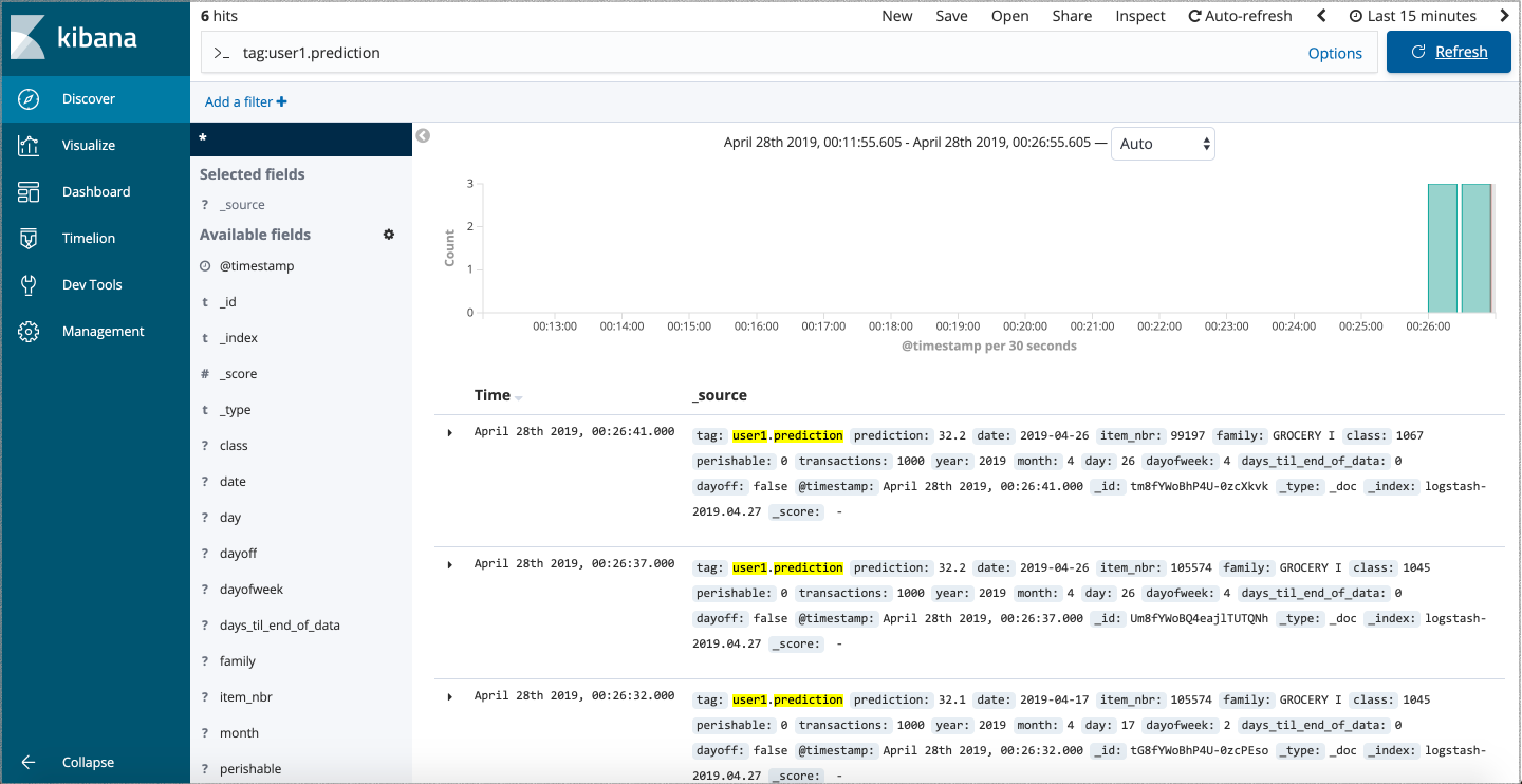
Figure 9: analysing our model's predictions against real input data in Kibana
There are other popular monitoring and observability tools, such as the ELK stack (a variation that uses Logstash instead of FluentD for log ingestion and forwarding), Splunk, among others.
Collecting monitoring and observability data becomes even more important when you have multiple models deployed in production. For example, you might have a shadow model to assess, you might be performing split tests, or running multi-arm bandit experiments with multiple models.
This is also relevant if you are training or running federated models at the edge — e.g. on a user's mobile device — or if you are deploying online learning models that diverge over time as they learn from new data in production.
By capturing this data, you can close the data feedback loop. This is achieved either by collecting more real data (e.g. in a pricing engine or a recommendation system) or by adding a human in the loop to analyse the new data captured from production, and curate it to create new training datasets for new and improved models. Closing this feedback loop is one of the main advantages of CD4ML, as it allows us to adapt our models based on learnings taken from real production data, creating a process of continuous improvement.
The End-to-End CD4ML Process
By tackling each technical challenge incrementally, and using a variety of tools and technologies, we managed to create the end-to-end process shown in Figure 10 that manages the promotion of artifacts across all three axis: code, model, and data.
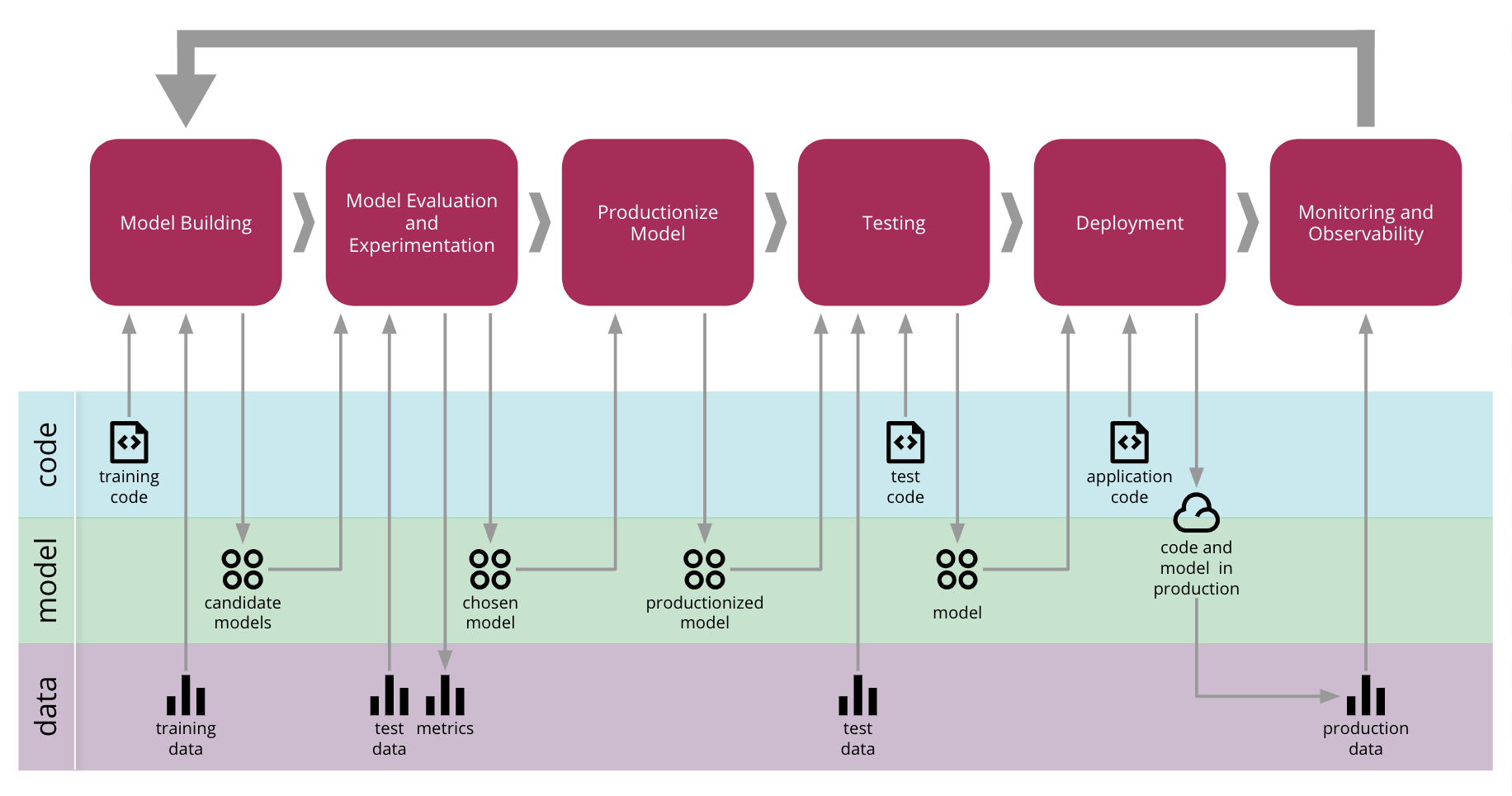
Figure 10: Continuous Delivery for Machine Learning end-to-end process
At the base, we need an easy way to manage, discover, access, and version our data. We then automate the model building and training process to make it reproducible. This allows us to experiment and train multiple models, which brings a need to measure and track those experiments. Once we find a suitable model, we can decide how it will be productionized and served. Because the model is evolving, we must ensure that it won't break any contract with its consumers, therefore we need to test it before deploying to production. Once in production, we can use the monitoring and observability infrastructure to gather new data that can be analysed and used to create new training data sets, closing the feedback loop of continuous improvement.
A Continuous Delivery orchestration tool coordinates the end-to-end CD4ML process, provisions the desired infrastructure on-demand, and governs how models and applications are deployed to production.
Where do We Go From Here?
The example application and code we used in this article is available on our Github repository, and was used as the basis for a half-day workshop that we presented at various conferences and at our clients. We continue to evolve our ideas about how to implement CD4ML. In this section we conclude by highlighting some areas of improvement that are not reflected in the workshop material, as well as some open areas that require further exploration.
Data Versioning
In Continuous Delivery, we treat every code commit as a release candidate, which triggers a new execution of the deployment pipeline. Assuming that commit passes through all the pipeline stages, it can be deployed to production. When talking about CD4ML, one of the regular questions we get is “how can I trigger a pipeline when the data changes?”
In our example, the Machine Learning pipeline in Figure 5 starts with the download_data.py
file, which is responsible for downloading the training dataset from a
shared location. If we change the contents of the dataset in the shared
location, it won't immediately trigger the pipeline, as the code has not
changed and DVC won't be able to detect it. To version the data we would
have to create a new file or change the file name, which in turn would
require us to update the download_data.py script with the
new path and therefore create a new code commit.
An improvement to this approach would be to allow DVC to track the file content for us, by replacing our hand-written download script with:
dvc add data/raw/store47-2016.csv ➊
This will slightly change the first step of our Machine Learning pipeline, as shown in Figure 11.
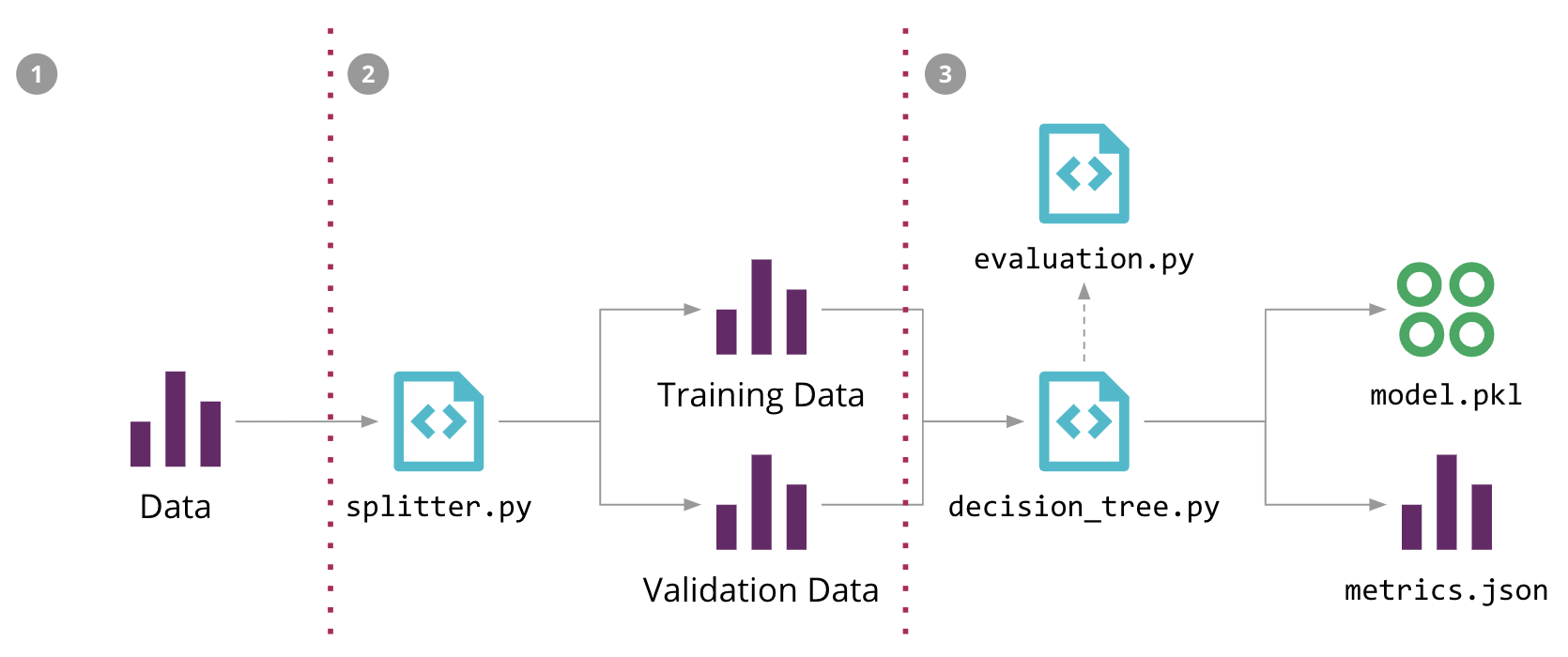
Figure 11: updating the first step to allow DVC to track the data versions and simplifying the ML Pipeline
This creates a metadata file that tracks a checksum of the file's content which we can commit to Git. Now when the file contents change, the checksum will change and DVC will update that metadata file, which will be the commit we need to trigger a pipeline execution.
While this allows us to retrain our model when the data changes, it doesn't tell the entire story about data versioning. One aspect is data history: ideally you would want to keep an entire history of all data changes, but that's not always feasible depending on how frequently the data changes. Another aspect is data provenance: knowing what processing step caused the data to change, and how that propagates across different data sets. There is also a question around tracking and evolving the data schema over time, and whether those changes are backwards and forwards compatible.
If you are in a streaming world, then these aspects of data versioning become even more complicated to reason about, so this is an area where we expect more practices, tools and techniques to evolve.
Data Pipelines
Another aspect we haven't covered so far is how to version, test, deploy, and monitor the data pipelines themselves. In the real world, some tooling options are better than others to enable CD4ML. For example, many ETL tools that require you to define transformation and processing steps through a GUI, are usually not easy to version control, test, or deploy to hybrid environments. Some of them can generate code that you can treat as an artifact and put through a deployment pipeline.
We tend to prefer Open Source tools that allow us to define the Data Pipelines in code, which is easier to version control, test, and deploy. For example, if you are using Spark, you might have your data pipeline written in Scala, you can test it using ScalaTest or spark-testing-base, you can package the job as a JAR artifact that can be versioned and deployed on a Deployment Pipeline in GoCD.
As Data Pipelines are usually either running as a batch job or as a long-running streaming application, we didn't include them in the end-to-end CD4ML process diagram in Figure 10, but they are also another potential source of integration issues if they change the output that either your model or your application expect. Therefore, having integration and data Contract Tests as part of our Deployment Pipelines to catch those mistakes is something we strive for.
Another type of test that is relevant for Data Pipelines is a data quality check, but this can become another extensive topic of discussion, and is probably better to be covered in a separate article.
Platform Thinking
As you might have noticed, we used various tools and technologies to implement CD4ML. If you have multiple teams trying to do this, they might end up reinventing things or duplicating efforts. This is where platform thinking can be useful. Not by centralizing all the efforts in a single team that becomes a bottleneck, but by focusing the platform engineering effort into building domain-agnostic tools that hide the underlying complexity and speed up teams trying to adopt it. Our colleague Zhamak Dehghani covers this in more detail on her Data Mesh article.
Applying platform thinking to CD4ML is why we see a growing interest in Machine Learning platforms and other products that are trying to provide a single solution to manage the end-to-end Machine Learning lifecycle. Many of the major technology giants have developed their own in-house tools, but we believe this is an active area of research and development, and expect new tools and vendors to appear, offering solutions that can be more widely adopted.
Evolving Intelligent Systems without Bias
As soon as your first Machine Learning system is deployed to production, it will start making predictions and be used against unseen data. It might even replace a previous rules-based system you had. It is important to realise that the training data and model validation you performed was based on historical data, which might include inherent bias based on how the previous system behaved. Moreover, any impact your ML system might have on your users going forward, will also affect your future training data.
Let's consider two examples to understand the impact. First, let's consider the demand forecasting solution we explored throughout this article. Let's assume there is an application that takes the predicted demand to decide the exact quantity of products to be ordered and offered to customers. If the predicted demand is lower than the actual demand, you will not have enough items to sell and therefore the transaction volume for that product decreases. If you only use these new transactions as training data for improving your model, over time your demand forecast predictions will degrade.
For the second example, imagine that you are building an anomaly detection model to decide if a customer's credit card transaction is fraudulent or not. If your application takes the model decision to block them, over time you will only have “true labels” for the transactions allowed by the model and less fraudulent ones to train on. The model's performance will also degrade because the training data becomes biased towards “good” transactions.
There is no simple solution to this problem. On our first example, retailers also consider out-of-stock situations and order more items than forecasted to cover a potential shortage. For the fraud detection scenario, we can ignore or override the model's classification sometimes, using some probability distribution. It is also important to realise that many datasets are temporal, i.e. their distribution changes over time. Many validation approaches that perform a random split of data assume they are i.i.d. (independent and identically distributed), but that is not true once you consider the effect of time.
Therefore, it is important to not just capture the input/output of a model, but also the ultimate decision taken by the consuming application to either use or override the model's output. This allows you to annotate the data to avoid this bias in future training rounds. Managing training data and having systems to allow humans to curate them is another key component that will be required when you face these issues.
Evolving an intelligent system to choose and improve ML models over time can also be seen as a meta-learning problem. Many of the state of the art research in this area is focused on these types of problems. For example, the usage of reinforcement learning techniques, such as multi-arm bandits, or online learning in production. We expect that our experience and knowledge on how to best build, deploy, and monitor these types of ML systems will continue to evolve.
Conclusion
As Machine Learning techniques continue to evolve and perform more complex tasks, so is evolving our knowledge of how to manage and deliver such applications to production. By bringing and extending the principles and practices from Continuous Delivery, we can better manage the risks of releasing changes to Machine Learning applications in a safe and reliable way.
Using a sample sales forecasting application, we have shown in this article the technical components of CD4ML, and discussed a few approaches of how we implemented them. We believe this technique will continue to evolve, and new tools will emerge and disappear, but the core principles of Continuous Delivery remain relevant and something you should consider for your own Machine Learning applications.
Acknowledgments
First of all, thanks to Martin Fowler for helping us redefine the narrative and structure of this article, and for hosting it.
Special thanks to many current and former ThoughtWorkers who have been helping us create and distill the ideas in this article through our workshops and client work, including Arun Manivannan, Danni Yu, David Tan, Emily Gorcenski, Emma Grasmeder, Jin Yang, Jonathan Heng, and Juan López.
Also thanks to the following early reviewers who provided invaluable feedback on the first draft of this article: Chris Ford, Fabio Kung, Fernando Meyer, Guilherme Silveira, Kyle Hodgson, and Rodrigo Kumpera.
Footnotes
1: There are efforts around AutoML to create methods and tools to automate many of the steps in the ML development process.
2: There is active research on tools and systems such as ease.ml/ci and ease.ml/meter to help manage and understand when new test data is required, or when models are overfitting.
Significant Revisions
19 September 2019: Published final installment
18 September 2019: Published installment on data versioning and data pipelines
11 September 2019: Published installment with orchestration and observability.
09 September 2019: Published installment with experiments tracking and model deployment.
06 September 2019: Published installment with model serving and testing
04 September 2019: published installment with discoverable data and reproducible training
03 September 2019: published first installment: introduction and challenges